![]()
The following vignette describes the theory and usage of TimeCycle.
For a comprehensive analysis and discussion of TimeCycle’s performance in detecting rhythmic genes, see the accompanying paper.
For details pertaining to the data and source code used in the analysis, see the
nesscoder/TimeCycle-datagit repository.
Theory
Algorithm Design Overview
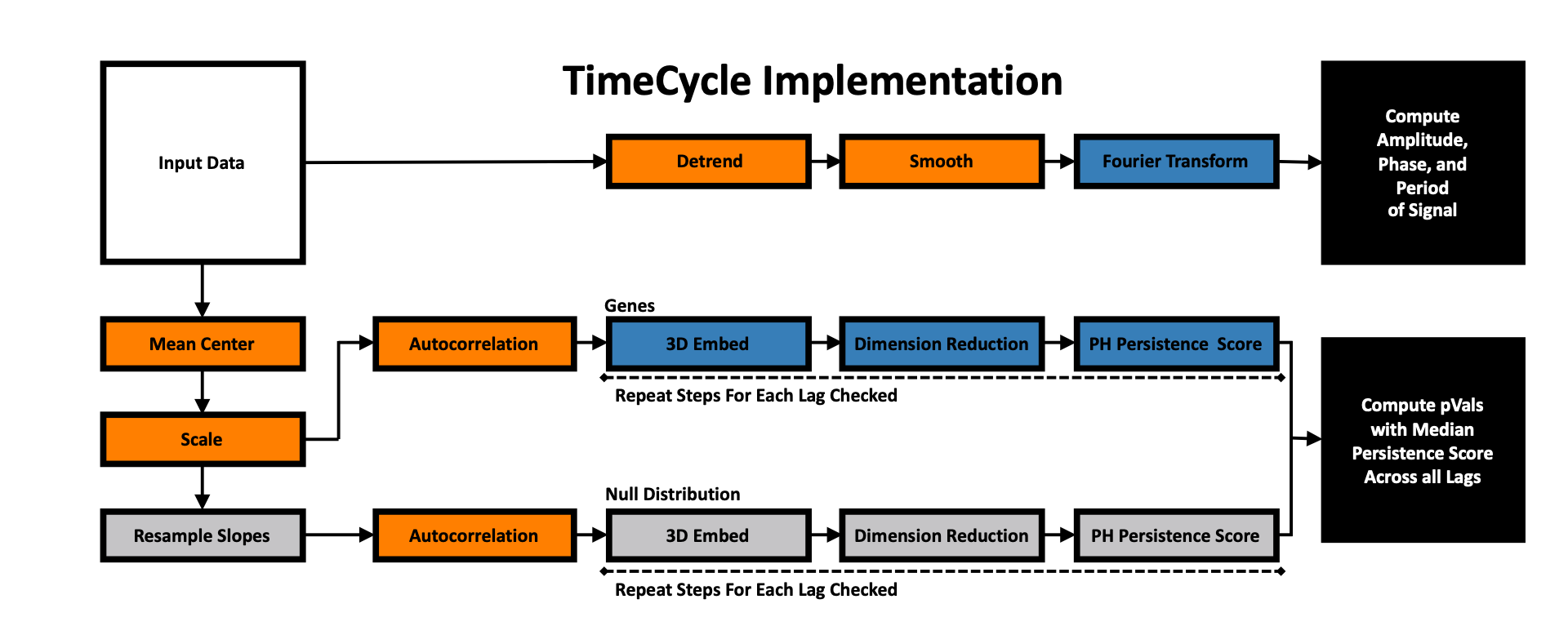
TimeCycle was developed as a reference-free method to quantify and classify cycling from non-cycling expression patterns in transciptomic time-series data. The basic algorithm framework is divided into two independent analyses: cycle detection and parameter estimation. The cycle detection framework consists of a rescaling/normalization step, reconstruction of the state space via 3-D time-delayed embedding, non-linear dimension reduction to remove trends, quantification of the measure of circularity via persistent homology, and comparison of that measure to a bootstrapped null distribution of resampled time-series to assess statistical significance. The period estimation framework consists of a preprocessing step (i.e. detrending and smoothing) followed by period, amplitude, and phase estimations via a Fourier transfrom fitting procedure. A complete description pertaining to each step in the TimeCycle method is found below.
Takens’ Theorem
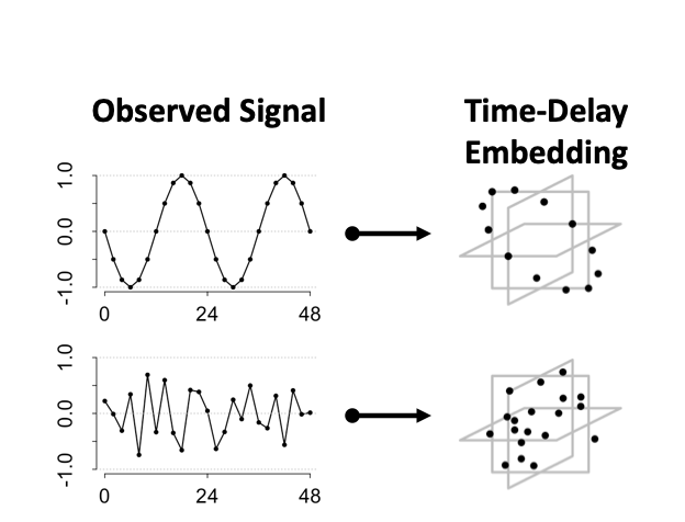
TimeCycle utilizes Takens’ Theorem — dynamical systems theory — to deconvolve rhythmic signals from non-rhythmic signals. Takens’ theorem proves that all the information needed to reconstruct the state space of a multivariate dynamic system can be captured by the embedded time-series of a single variable (Takens, 1981). As a consequence of the this larger theory, it was shown that the dynamics of a periodic signal exhibit circular patterns in the embedded space.
An embedded periodic function forms a circle.
An embedded non-periodic function forms a mass.
We can exploit this property for cycling detection by quantifying the circularity of data in the time-delay embedded space.
3-D Time-Delay Embedding
Takens’ Theorem asserts that to reconstruct the state space (\(S\)) from a single time-series, define a lag constant \(T\) to generate a vector of delayed coordinates and plot the signal in the embedded space against the delayed version of itself. TimeCycle uses a 3-D embedding to encapsulate more dynamical history and enable periodic and non-periodic components to be separated. Above we show the constructed manifold when setting the lag \(T = 3\).
\[ S=\begin{cases} \color{blue}{\mathbf{x}}&= f(t)\\ \mathbf{y}&= f(t+T)\\ \color{orange}{\mathbf{z}}&= f(t+2T) \end{cases} \]
While the theorem proves the dynamics of the systems are preserved in the state space, the choice of lag \(T\) to optimally reconstruct the state space manifold is unknown; since the organization depends on the choice of lag relative to the sampling scheme. As a result, TimeCycle sweeps through a series of lagged time-delays — by default from \(T = 2\) to \(T = 5\) — and computes the degree of circularity across the generated manifolds. If a signal is truly rhythmic, on average the state space manifold across lags should still maintain circular dynamics.
Detrending Via Dimension Reduction
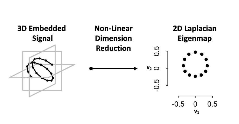
An important part of cycle detection is detrending non-rhythmic artifacts, such as linear trends, from time-series. A common and logical approach is to fit a line to the time-series and subtract out the fit prior to cycle detection. While this removes linear trends, the detrending procedure introduces false positives, as previously non-rhythmic signals — e.g. sigmoidal and exponential — look rhythmic. TimeCycle uses the state space to detrend signals without introducing detrending artifacts. Rather then going straight to a 2-D embedding and preserving the trend in the state space manifold, TimeCycle opts to transformed the signal into a 3-D embedding and remove trending artifacts during the dimension reduction step prior to the persistence calculation. For example:
Dampened and trending signals form spirals and helices in the embedded space
Non-LinearDimension Reduction — Laplacian Eigenmap — is used to articulate the underlying circular manifold.
As helices maintain a cyclic pattern at an adjusted point in space, the Laplacian Eigenmap preserves the local circular geometry of the 3-D helix in a 2-D space.
By removing the linear component, the circular (periodic) component is recovered.
As non-rhythmic signals by definition do not form circular dynamics in the embedded space, the dimension reduction limits the introduction of false positives as previously observed in other methods.
Persistent Homology
𝜖
Persistent homology is an algebraic way to measure shape invariant (i.e. components, holes, voids, and higher dimensional analogs) about a discrete set of points. The algorithmic outline can be described as follows:
Goal:
- Parameterize circularity of the embedded points by computing a persistence score (\(PS\)).
Method:
From each point of the embedded signal, a circle of radius \(\epsilon\) is incrementally grown
Connect points if they are at least a diameter \(2\epsilon\) apart.
A topological cycle appears at some \(\epsilon_{birth}\) and disappears at \(\epsilon_{death}\).
\(PS = \epsilon_{death} - \epsilon_{birth}\)
More circular embeddings have larger difference between events. As a consequence of Takens’ Theorem, periodic signals will have high persistence, while non-periodic signals have low persistence. This difference in persistence scores allows for a quatitatie classification of rhythmic and non-rhythmic signals.
The Null Distribution
A major issue with current non-parametric cycle detection methods are the use of unrealistic null distributions. Non-parametric methods bootstrap a null distribution by generating random time-series sampled from a Gaussian distribution. In practice, gene expression in the biological context are constrained by transcription and degradation rates, and thus an assumption of random-independent Gaussian noise is inappropriate as it allows for chance fluctuations outside the realm of biological possibility. TimeCycle bootstraps times-series from changes in gene expression between sampled time-points — modeling biological transcription and degradation constraints.
Goal:
- Generate Biologically relevant null distribution for hypothesis testing
Method:
Construct null distribution from resampling of observed data
Compute difference between consecutive time-points in observed data
Resample differences with replacement to form random time-series
Compare persistence between observed and resampled time-series
Significance Definition:
- By random chance, how often will you see a gene cycling with a persistence — averaged across a range of frequency (i.e. lags) — as or more extreme than the observed gene’s persistence.
Pre-Processing and Normalization For Computational Efficiency
As stated in the algorithm design overview, TimeCycle is divided into two independent analyses: Cycle detection and parameter estimation. In the cycle detection analysis, genes are mean center and scaled; removing variation as a result of expression. By scaling gene expression, the same null distribution can be used for significance testing across all genes — decreasing the computation load in comparison to the alternative of not scaling and needing to generate a null distribution for each gene. When performing the less computationally costly parameter estimation, the rescaling procedure is omitted to preserve amplitude measures.
FFT Period Estimation
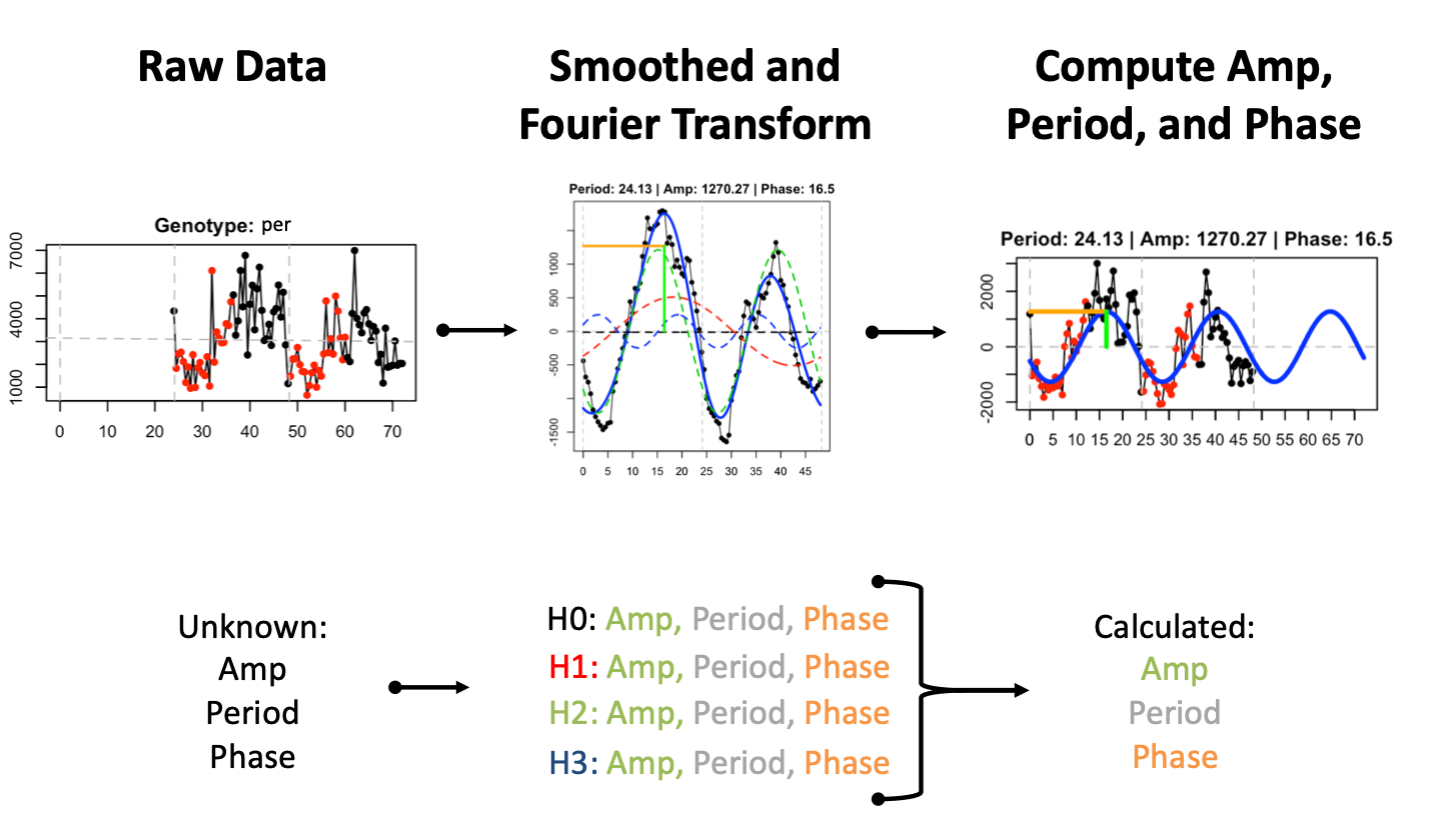
As described above, parameter estimation is performed independent of the cycling detection analysis. Prior to estimation, signals are linearly detrended and smoothed via a moving average before computing the signal fit (Middle Panel - blue solid line) using the first three harmonics (Middle Panel - red, green, and blue dashed lines) of the fast Fourier transform (FFT). The FFT fit is used to compute the amplitude, period, and phase of oscillation (Right Panel - green, grey, and orange lines, respectively). A reconstructed model for the oscillation using the parameter estimates (Right Panel - blue solid line) is overlaid on the original signal in the right panel .
Usage
Input Data Structure
Keeping with convention of other cycling detection methods, TimeCycle takes as input a data.frame of numeric gene expression values over time (row = genes x col = ZT times).
Specify the genes names in the row names
Specify the ZT in the column names
# Pseudo code
# df = data.frame of expression values (genes x time point)
# geneNames = a vector that holds the name of each gene

ztTimes <- seq(from = 0, to = 48, by = 2)
colnames(df) <- paste0("ZT_", ztTimes)
rownames(df) <- geneNames
A properly formatted data.frame should look as follows:
| ZT_0 | ZT_2 | … | ZT_46 | ZT_48 | |
| gene_1 | 1.0 | 3.0 | … | 7.0 | 4.0 |
| gene_2 | 4.0 | 8.0 | … | 2.0 | 1.0 |
| ⋮ | ⋮ | ⋮ | ⋱ | ⋮ | ⋮ |
| gene_n-1 | 5.0 | 8.0 | … | 3.0 | 2.0 |
| gene_n | 9.0 | 4.0 | … | 7.0 | 3.0 |
Replicate Labels
Even Replicates
Following the convention above, the input data.frame should define the gene names and ZT times with replicate ZT times (i.e. R1, R2, …) placed next to each other.
A properly formatted data.frame with even replicates across all time-points should look as follows:
| ZT_0_R1 | ZT_0_R2 | ZT_2_R1 | ZT_2_R2 | … | ZT_46_R1 | ZT_46_R2 | ZT_48_R1 | ZT_48_R2 | |
| gene_1 | 1.0 | 2 | 3.0 | 2.0 | … | 7.0 | 9.0 | 4.0 | 5.0 |
| gene_2 | 4.0 | 3 | 8.0 | 9.0 | … | 2.0 | 1.0 | 1.0 | 3.0 |
| ⋮ | ⋮ | ⋮ | ⋮ | ⋮ | ⋱ | ⋮ | ⋮ | ⋮ | ⋮ |
| gene_n-1 | 5.0 | 6 | 8.0 | 7.0 | … | 3.0 | 4.0 | 2.0 | 1.0 |
| gene_n | 9.0 | 8.0 | 4.0 | 5.0 | … | 7.0 | 8.0 | 3.0 | 2.0 |
Example Replicate Labels
With even replicates, the number of replicates at each ZT time should be explicitly specified in a vector — e.g. a data set with 2 replicates at 24 different ZT times would have a replicate label vector of length 24, even through there are 48 samples total:
# Each ZT time point in the data.frame has 2 replicates
replicateLabels_even <- rep(x = 2, times = ncol(df_evenReplicates)/2)

# Run TimeCycle with default setting
TimeCycle(data = df_evenReplicates, repLab = replicateLabels_even)
In the case of zhang2014() example data set — sampled every 2 hours for 48 hours (i.e. 24 ZT times) — there is only 1 sample per time point. As a result, the replicate label would have 1 sample for all 24 time points: replicateLabel <- rep(x = 1, times = ncol(zhang2014)).
Uneven Replicates
Following the convention above, the input data.frame should define the gene names and ZT times with replicate ZT times (i.e. R1, R2, …) placed next to each other.
A properly formatted data.frame with uneven replicates across all time-points should look as follows:
| ZT_0_R1 | ZT_0_R2 | ZT_0_R3 | ZT_2_R1 | … | ZT_46_R1 | ZT_46_R2 | ZT_48_R1 | ZT_48_R2 | |
| gene_1 | 1.0 | 2.0 | 1.0 | 3.0 | … | 7.0 | 9.0 | 4.0 | 5.0 |
| gene_2 | 4.0 | 3.0 | 5.0 | 8.0 | … | 1.0 | 1.0 | 1.0 | 3.0 |
| ⋮ | ⋮ | ⋮ | ⋮ | ⋮ | ⋱ | ⋮ | ⋮ | ⋮ | ⋮ |
| gene_n-1 | 5.0 | 6.0 | 4.0 | 8.0 | … | 3.0 | 4.0 | 2.0 | 1.0 |
| gene_n | 9.0 | 8.0 | 9.0 | 4.0 | … | 7.0 | 8.0 | 3.0 | 2.0 |
Example Replicate Labels
With uneven replicates,the number of replicates at each ZT time should be explicitly specified in a vector — e.g. a data set with 24 different ZT times would have a replicate label vector of length 24, even through there may be more than 24 samples total. Do NOT include unsampled ZT time with 0 replicates.
# Pseudo code for example data.frame above
# Specify the number or replicates for each ZT time point in the data.frame
# ... = replicate values at omited ZT times. Actual code must specify.
replicateLabel_uneven <- c(3,1,...,2,2)

length(replicateLabel_uneven)
#> 24

# Run TimeCycle with default setting
TimeCycle(data = df_unevenReplicates, repLab = replicateLabels_uneven)
Missing Data
Missing data should be labeled with an NA. Use the same convention as above for defining replicate labels for data.frames with even and uneven number of replicates.
A properly formatted data.frame with missing values should look as follows:
| ZT_0 | ZT_2 | … | ZT_46 | ZT_48 | |
|---|---|---|---|---|---|
| gene_1 | 1.0 | NA |
… | 7.0 | 4.0 |
| gene_2 | 4.0 | 8.0 | … | NA |
1.0 |
| ⋮ | ⋮ | ⋮ | ⋱ | ⋮ | ⋮ |
| gene_n-1 | 5.0 | 8.0 | … | NA |
2.0 |
| gene_n | NA |
4.0 | … | 7.0 | 3.0 |
Parameter Selection
The main TimeCycle function’s parameters are defined by default for the minimal recommended sampling scheme of every 2-h for 48-h (Hughes et al., 2017; Laloum & Robinson-Rechavi, 2020; Ness-Cohn et al., 2020).
TimeCycle(
  data,
  repLabel,
  resamplings = 10000,
  minLag = 2,
  maxLag = 5,
  period = 24,
  cores = parallel::detectCores() - 2,
  laplacian = T,
  linearTrend = F
)
For defining the data and repLabel inputs, see Input Data Structure and Replicate Labels section above. The default parameters are recommended for all sampling schemes that meet the minimal recommended sampling requirements.
For Time-series sampled:
we recommend setting maxLag = 3, rather than the default maxLag = 5. See sections below for details.
⚠️ Warning: Data sets sampled under the minimal recommended sampling scheme of every 2-h for 48-h have been shown to be unreliable across cycling detection methods (Hughes et al., 2017; Laloum & Robinson-Rechavi, 2020; Ness-Cohn et al., 2020) ⚠️
Short Time-Series
While we do NOT recommend using a sampling scheme less than 48-h in length; for these data sets use maxLag = 3, rather than the default maxLag = 5. Furthermore, TimeCycle requires a minimum of 18 time points for cycling detection — ie. a sampling scheme of every 2-h for 36-h.
Often researchers elect to use a 24-h sampling scheme; however circadian cycling detection methods have been shown to be unreliable at this sampling length — i.e. a lack of reproducibility. The lack of reproducibility comes from the fact that the sampling scheme is inherently under-sampled for determining a circadian rhythm — a cycle that repeats with a 24-h period. Methods that use a curve fitting procedure classify a gene as cycling or not, depending on if the 24-h of data match up with the dynamics of the reference curve (i.e. sin wave). Nonetheless, classifying this signal as circadian is illogical, as there is no information as to what happens to a gene in the next 24-h — if it repeats the cycle or has some other dynamics. When this data is processed by TimeCycle, this lack of information presents itself in the inability to reconstruct a cycle in the embedded space — thus all genes are classifies as non-cycling. This logically makes sense since we do not have enough information to know what happens to the signal after the first 24-h period and thus by definition cannot call a gene circadian or not. See TimeCycle’s supplement for details.
At the 36-h every 2-h minimum, we now have information pertaining to 1.5 cycles — enough to at least make a prediction about the signal dynamics in the next 24-h window. Users may still see decreased performance in detection of non-symmetric cyclers. Nonetheless, strong symmetric cyclers and know circadin genes can still be detected at 36-h. See TimeCycle paper for details.
Sparsely Sampled Data
While we do NOT recommend using a sampling interval less frequent than every 2-h; for these data sets use maxLag = 3, rather than the default maxLag = 5. Note that circadian cycling detection methods, as well as TimeCycle, have been shown to be unreliable at 4-h intervals and above — i.e. lack of reproducibility with high false positives rates (Hughes et al., 2017; Ness-Cohn et al., 2020)
The depreciation in TimeCycle’s performance is attributed to a sparsely-sampled manifolds in the state space, potentially resulting in an insufficient number of data-points for cycle formation. At higher lags, more points are removed from the embedded manifold, thus by setting the maxLag = 3, we decrease the chances of having an insufficient number of data-points for cycle formation.
Prioritize Detection of Linear Trending Signals
⚠️ Warning: Setting linearTrend = T may increase false positive rates - Not Recommended - Use with Caution ⚠️
TimeCycle has been shown to have decreased performance in detecting linear trending signals for time-series sampled longer than 48-h. As time-series sampling is extended, linear and damped oscillatory trends become more pronounced — dominating the underlying signal and hindering detrending in the state space. Excluding trending signals can be (un)desirable depending on the oscillatory patterns of interest in the context of the biological question being asked.
To prioritize the detection of linear trending signals with TimeCycle, set the linearTrend = T.
In this case, TimeCycle processes the derivative the autocorrelation function before preforming the topological analysis. This process removes the linear trend, while persevering the oscillatory dynamics.
While this preprocessing step improves the detection of linear trending oscillations, the process introduces the risk of false positives, as previously non-rhythmic signals may look rhythmic — similar to the short coming of other cycling detection methods. If proceeding wih this parameter selection, we recommend checking the genes detected as cycling — as this process will detect sigmoidal waveforms that shift at the 24 hour mark as cycling.